Mastering the SUMIFS Function in Microsoft Excel for Conditional Summing with Multiple Criteria

The SUMIFS function in Microsoft Excel is a conditional sum function used to add up cells based on multiple conditions.
The syntax for the SUMIFS function is as follows:

SYNTAX

SUMIFS(sum_range, criteria_range1, criteria1, [criteria_range2, criteria2, ...])

sum_range: the range of cells to be summed
criteria_range1:the first range of cells to be evaluated based on criteria1
criteria1: the first criteria to be used in the evaluation
criteria_range2, criteria2, ...: optional additional ranges and criteria to be evaluated

Example

Display Year and Month Wise Report

S.No	Year	Month	Product	Sales
1	2021	January	PEN	5896
2	2020	February	PENCIL	7542
3	2020	January	PEN	1200
4	2021	January	PENCIL	2500
5	2021	February	NOTE	6500
6	2020	February	NOTE	6500

=SUMIFS(E3:E8,B3:B8,2021,C3:C8,"January")

Output

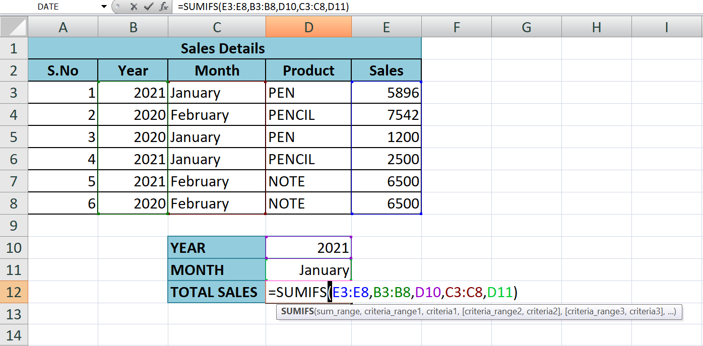
The SUMIFS function in the above formula calculates the sum of cells in the range E3:E8 based on multiple criteria.

E3:E8 is the sales amount (sum_range), which is the range of cells to be summed.
B3:B8 is the first criteria_range its carry the sales year data, which is the range of cells to be evaluated based on the first criteria.
2021 is the first criteria, which is used to evaluate the values in the first criteria_range. The formula will sum only the values in the sum_range where the corresponding values in the criteria_range1 are equal to 2021.
C3:C8 is the second criteria_range its carry the details of sales month, which is used to evaluate the values in the second criteria.
"January" is the second criteria, which is used to evaluate the values in the second criteria_range. The formula will sum only the values in the sum_range where the corresponding values in the second criteria_range are equal to "January"..

So, this formula calculates the sum of cells in E3:E8 only where the corresponding values in B3:B8 are equal to 2021 and the corresponding values in C3:C8 are equal to "January".