AVERAGEIFS Function - Calculate the Average Based on Multiple Criteria

The AVERAGEIFS function is a built-in mathematical function in spreadsheet software, such as Microsoft Excel or Google Sheets. It allows you to calculate the average of a range of cells that meet multiple criteria.

Syntax

AVERAGEIFS(average_range, criteria_range1, criteria1, criteria_range2, criteria2, ...)

Where:

average_range: This is the range of cells that you want to calculate the average for. It can be a single column or row, or a combination of multiple columns or rows.
criteria_range1, criteria_range2, ...: These are the ranges of cells that contain the criteria you want to apply for averaging. You can specify up to 127 pairs of criteria_range and criteria.
criteria1, criteria2, ...: These are the criteria that you want to apply to the corresponding criteria_range. The criteria can be a number, text, logical expression, or cell reference.

The AVERAGEIFS function calculates the average of only those cells in the average_range that meet all the specified criteria. It excludes any cells that do not meet the criteria or contain text, empty values, or errors.

Using the AVERAGEIFS function is helpful when you need to calculate an average based on multiple conditions. For example, you can use it to find the average sales of a specific product within a certain time period or calculate the average score of students who meet certain criteria, such as being from a specific city and having a grade above a certain threshold.

By using the AVERAGEIFS function, you can easily analyze data and obtain more precise averages based on specific conditions.

The formula "=AVERAGEIFS(C3:C15, A3:A15, "South", B3:B15, "January")" calculates the average sales for the month of January in the South region.

Here's how the formula works:

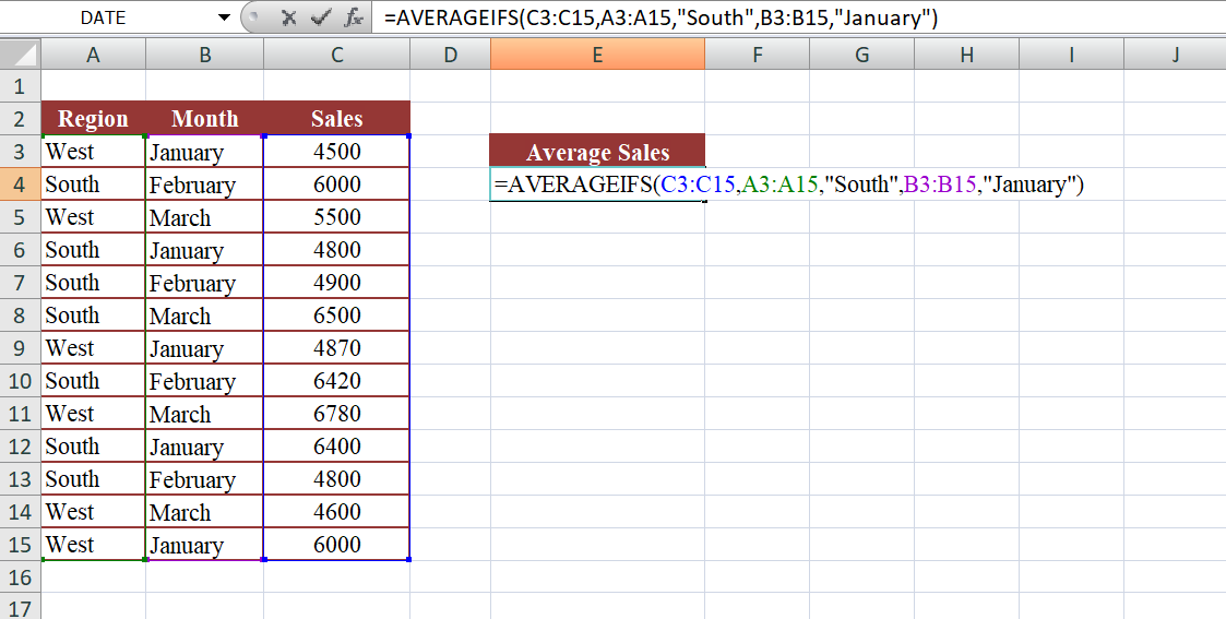
"C3:C15" represents the range of cells containing the sales values.
"A3:A15" represents the range of cells containing the region values.
"B3:B15" represents the range of cells containing the month values.
"South" is the criteria applied to the region column.
"January" is the criteria applied to the month column.

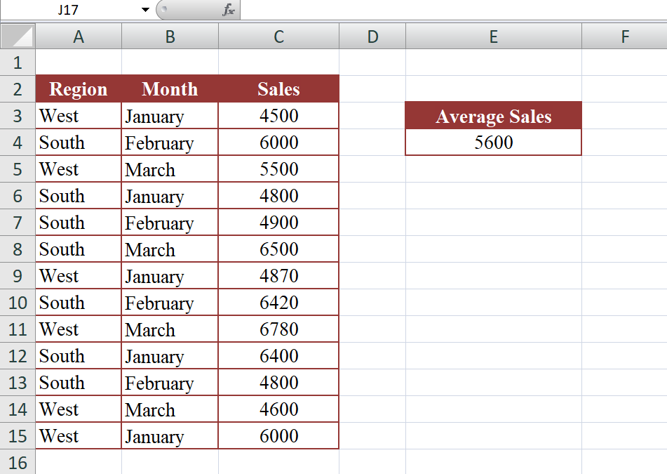
The AVERAGEIFS function will consider only those sales values that meet both criteria (South region and January month) and calculate their average. In the provided data, the formula will consider cells C4, C10, and C11 since they correspond to the South region in the month of January.

Therefore, the result of the formula "=AVERAGEIFS(C3:C15, A3:A15, "South", B3:B15, "January")"will be the average of those three sales values, which is approximately 5600.