AVERAGEIF Function: Calculating the Average of Values Based on a Condition in Spreadsheets
The AVERAGEIF function is a mathematical function commonly used in spreadsheet programs like Microsoft Excel or Google Sheets. It calculates the average of a range of values based on specified criteria or conditions.
Syntax
AVERAGEIF(range, criteria, [average_range])
Where:
- range: This is the range of cells or a column or a row from which you want to evaluate the values. The AVERAGEIF function will check the values in this range against the specified criteria.
- criteria: This is the condition or criteria that the values in the range must meet to be included in the average calculation. It can be expressed using comparison operators like "=", ">", "<", ">=", "<=", "<>", or using wildcards like "*", "?".
- average_range (optional): This argument specifies the range of cells or a column or a row that contains the values you want to average. If this argument is omitted, the AVERAGEIF function will use the same range as the range argument for the average calculation.
The AVERAGEIF function is a mathematical function commonly used in spreadsheet programs like Microsoft Excel or Google Sheets. It calculates the average of a range of values based on specified criteria or conditions.
METHOD 1
Here's how the calculation works:
- Range of Values: First, you need to specify the range of values for which you want to calculate the average. This can be a range of cells, a column, or a row.
- Condition: You also need to provide a condition or criteria that the values must meet to be included in the average calculation. This condition can be based on specific values, expressions, or logical operators.
- Calculation: The AVERAGEIF function evaluates each value in the range against the specified condition. It includes only the values that meet the condition in the average calculation.
- Result: The AVERAGEIF function returns the average of the values that satisfy the specified condition.
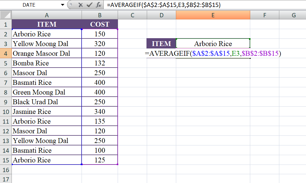
In the given example, there are two columns: "ITEM" and "COST." The "ITEM" column contains various food items, and the "COST" column contains their corresponding prices.
To calculate the average cost of a specific item, let's take "Arborio Rice" as an example. In this case, you can use the formula "=AVERAGEIF($A$2:$A$15,E3,$B$2:$B$15)".
- $A$2:$A$15: This represents the range of cells in column A (ITEM) where the criteria will be checked. It includes the items "Arborio Rice," "Yellow Moong Dal," and so on.
- E3: This is the specific criterion or condition that values in column A need to match. In this case, E3 refers to a cell that contains the text "Arborio Rice."
- $B$2:$B$15: This represents the range of cells in column B (COST) from which the corresponding values will be averaged if they meet the specified criterion.
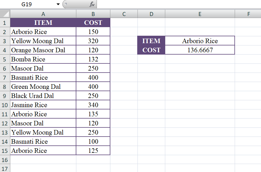
Using the given data, the formula will calculate the average cost of "Arborio Rice" as follows:
- "=AVERAGEIF($A$2:$A$15,E3,$B$2:$B$15)"
- "=AVERAGEIF($A$2:$A$15,"Arborio Rice",$B$2:$B$15)"
- "=AVERAGE(150, 135, 125)"
- "=136.67"
Therefore, the average cost of "Arborio Rice" based on the given data is approximately 136.67.
Output
METHOD 2
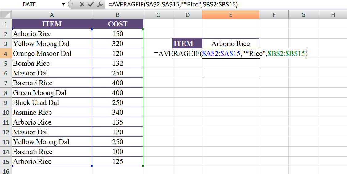
The formula "=AVERAGEIF($A$2:$A$15,"*Rice",$B$2:$B$15)" calculates the average cost of items that have "Rice" in their name based on the given data.
Let's break down the formula:
- $A$2:$A$15: This represents the range of cells in column A (ITEM) where the criteria will be checked. It includes the items "Arborio Rice," "Bomba Rice," "Basmati Rice," and "Jasmine Rice."
- "Rice": This is the specific criterion or condition that values in column A need to match. The asterisk () is a wildcard character that represents any number of characters, so "* Rice" matches any item in column A that ends with "Rice."
- $B$2:$B$15: This represents the range of cells in column B (COST) from which the corresponding values will be averaged if they meet the specified criterion.
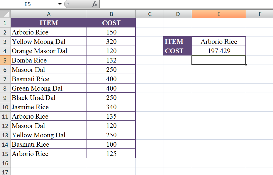
Using the given data, the formula will calculate the average cost of items ending with "Rice" as follows:
- "=AVERAGEIF($A$2:$A$15,"*Rice",$B$2:$B$15)"
- "=AVERAGEIF($A$2:$A$15,"*Rice",$B$2:$B$15)"
- "=AVERAGE(150, 132, 340, 135,100, 125)"
- "=197.3"
Therefore, the average cost of items ending with "Rice" based on the given data is approximately 197.3
Output
METHOD 3
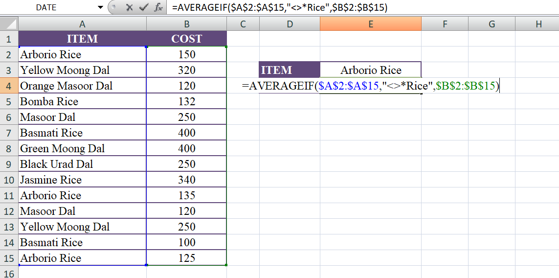
The formula "=AVERAGEIF($A$2:$A$15,"<>*Rice",$B$2:$B$15)" calculates the average cost of items that do not have "Rice" in their name based on the given data.
Let's break down the formula:
- $A$2:$A$15: This represents the range of cells in column A (ITEM) where the criteria will be checked. It includes the items "Arborio Rice," "Bomba Rice," "Basmati Rice," and "Jasmine Rice."
- "<>*Rice": This is the specific criterion or condition that values in column A need to match. The "<>" operator represents "not equal to," and "*Rice" matches any item in column A that ends with "Rice." So, "<>*Rice" matches any item that does not end with "Rice."
- $B$2:$B$15: This represents the range of cells in column B (COST) from which the corresponding values will be averaged if they meet the specified criterion.
Using the given data, the formula will calculate the average cost of items that do not end with "Rice" as follows:
- "=AVERAGEIF($A$2:$A$15,"<>*Rice",$B$2:$B$15)"
- "=AVERAGEIF($A$2:$A$15,"<>*Rice",$B$2:$B$15)"
- "=AVERAGE(320, 120, 250, 400, 400, 250, 120, 250)"
- "=275"
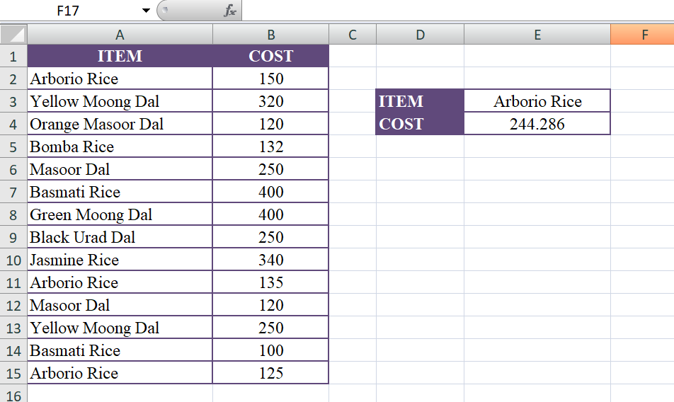
Therefore, the average cost of items that do not end with "Rice" based on the given data is 275.
Output
Learn All in Tamil © Designed & Developed By Tutor Joes | Privacy Policy | Terms & Conditions