Mastering the SUMIF Function in Excel: A Guide to Conditional Summation

The SUMIF function in Excel is used to calculate the sum of a range of values that meet a specific condition. It allows you to add up numbers based on a given criteria or condition. This can be particularly useful when you want to perform calculations on certain data points within a larger dataset.

The basic syntax of the SUMIF function is as follows:

Syntax

=SUMIF(range, criteria, [sum_range])

range: This is the range of cells that you want to evaluate based on the given criteria.
criteria: This is the condition that you want to apply to the cells in the specified range. It can be a value, expression, or text that defines which cells should be included in the sum.
sum_range: (Optional) This is the range of cells containing the actual values that you want to sum. If omitted, the range is used as the sum_range.

Advantages of Sumif Function

Conditional Summing: The primary advantage of the SUMIF function is its ability to perform conditional summing. It allows you to calculate the sum of values based on a specific condition or criteria. This is especially useful for quickly analyzing data subsets without the need for complex calculations.
Simplicity: The SUMIF function is relatively easy to use and understand. It doesn't require advanced formula knowledge, making it accessible to users with varying levels of Excel expertise.
Flexibility: You can use a wide range of criteria in the SUMIF function, including text, numbers, logical expressions, and wildcards. This flexibility enables you to perform calculations based on various conditions.
Efficiency: SUMIF allows you to efficiently calculate sums for specific subsets of data. It can significantly save time compared to manual calculations or more complex formulas.

Disadvantages of Sum Function

Single Criterion: The most significant limitation of the SUMIF function is that it supports only a single criteria. If you need to sum values based on multiple conditions, you'll need to use more complex functions like SUMIFS or other methods.
Limited Advanced Logic: While SUMIF is straightforward, it might not suffice for more intricate logic requirements. For complex conditions or calculations, you might need to resort to nested functions or other Excel features.
Performance Issues: When working with large datasets, using SUMIF excessively can impact spreadsheet performance. More complex functions might be more efficient in handling extensive data.
Limited to Summing: The primary purpose of the SUMIF function is to perform summation. If you require other calculations or operations based on conditions, you might need to use additional functions or methods.
Maintainability: If you're dealing with multiple criteria or complex conditions, using a series of SUMIF functions can make your spreadsheet formula-heavy and harder to maintain. This can lead to potential errors and difficulties in troubleshooting.

The SUMIF Function in various ways:

Basic Summing: The SUMIF function allows you to add up values from a range that meet a specified condition. It's like a digital calculator that only adds numbers that satisfy a particular requirement.
Conditional Addition: Think of SUMIF as a specialized calculator that follows rules. It checks each number in a list and adds only those that fit a given rule or condition.
Data Filter and Sum: Consider SUMIF as a data filter that sorts through numbers, and then it performs the math on the ones that pass the filter. It's like having a shelf of books and choosing only the red ones to count their pages.
Smart Adding Machine: Imagine SUMIF as a smart adding machine that scans a set of numbers and adds up only the ones you tell it to, based on specific characteristics you specify.
Customized Totaling: Think of SUMIF as your personal tallying assistant. It calculates a total for you, but only for the items you mark with a certain label or description.
Criteria-Based Addition: Picture SUMIF as a digital accountant. It goes through your financial records and adds up expenses, but only for transactions that match a particular category you specify.
Conditional Aggregator: Consider SUMIF as a conditional aggregator. It combines values, but only those that fit within a defined set of criteria that you provide.
Dynamic Math with Filters: Imagine SUMIF as a mathematical tool that dynamically adapts to your data. It performs calculations, but it's smart enough to consider only the data you want, thanks to its built-in filters.
Customized Subtotaling: Think of SUMIF as a customizable subtotaling wizard. It helps you determine subtotals based on specific conditions, making data analysis a breeze.
Summing by Rule: Picture SUMIF as a rule-based summing mechanism. It evaluates data according to your rules and adds up the numbers that meet those rules.
Targeted Summation: Consider SUMIF as a precision tool for summation. It focuses on specific data points and accurately calculates the sum based on your criteria.
Smart Filtering and Addition: Imagine SUMIF as a tool that combines smart filtering with addition. It filters out unwanted data and then performs mathematical operations on the remaining data.

Example 1: Summing Values Based on a Single Criteria

Amount	Category
500	Electronics
300	Clothing
700	Electronics
450	Accessories
250	Electronics
600	Clothing
350	Electronics
800	Accessories

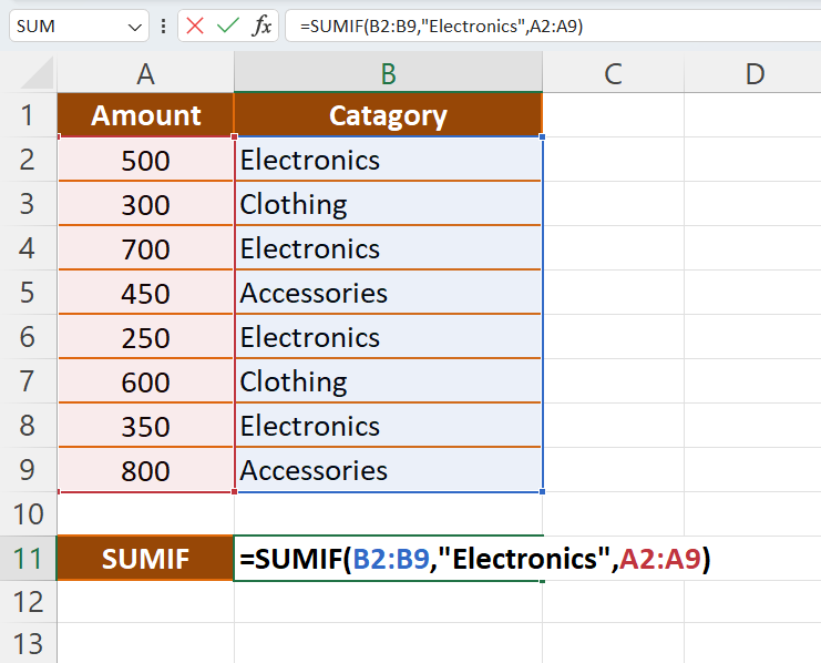
To calculate the total sales for the "Electronics" category using the SUMIF function, use this formula:

Syntax

=SUMIF(B2:B8, "Electronics", A2:A8)

You also have a formula "=SUMIF(B2:B9, "Electronics", A2:A9)" which calculates the sum of the "Amount" values for transactions that fall under the "Electronics" category.

Here's how the formula works step by step:

The formula starts by evaluating each cell in the "Category" column (B2 to B9) one by one.
It checks if the value in the "Category" column matches the condition "Electronics."
When it finds a match (in cells B2, B4, B5, and B7), it considers the corresponding value from the "Amount" column (A2 to A9).
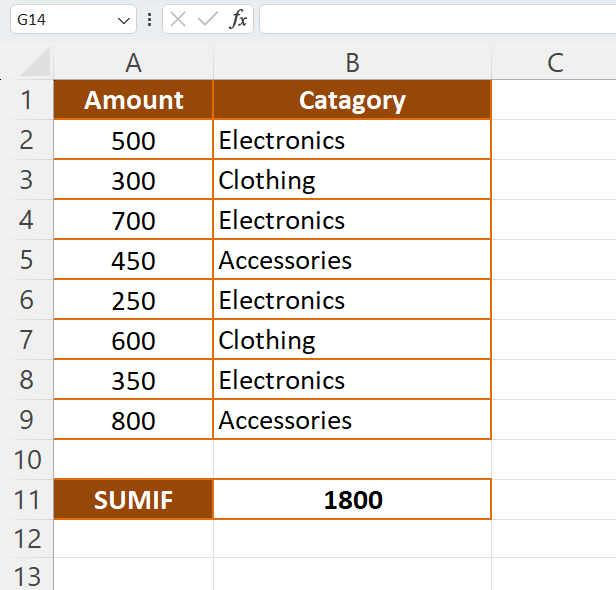
It adds up all the values from the "Amount" column that correspond to the "Electronics" category.

In your provided data, there are four transactions with the "Electronics" category and the corresponding amounts are 500, 700, 250, and 350. When you add these amounts together, you get a total of 1800.

So, the result of the formula "=SUMIF(B2:B9, "Electronics", A2:A9)" is 1800, which represents the total amount spent on transactions categorized as "Electronics."

This formula is a helpful way to quickly calculate the sum of values based on a specific condition in Excel or similar spreadsheet software. It's particularly useful when you want to analyze data and perform calculations based on certain criteria.

Output

Example 2: Summing Values Based on Numeric Criteria

Suppose you have a list of product quantities and prices in cells A1 to A8 and B1 to B8, respectively. You want to calculate the total cost of products with a price higher than $50.

Number 1	Number 2
5	40
3	60
8	70
2	45
6	55
4	30
7	80
1	90

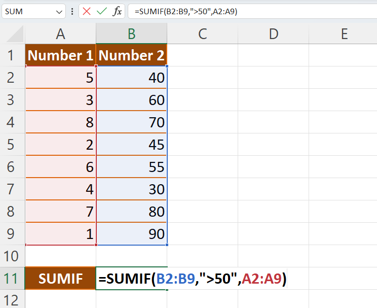
To calculate the total cost of products with a price higher than $50 using the SUMIF function, use this formula:

Syntax

=SUMIF(B1:B8, ">50", A1:A8)

You also have a formula "=SUMIF(B2:B9,">50",A2:A9)" which calculates the sum of "Number 1" values for pairs where the corresponding "Number 2" is greater than 50.

Here's how the formula works step by step:

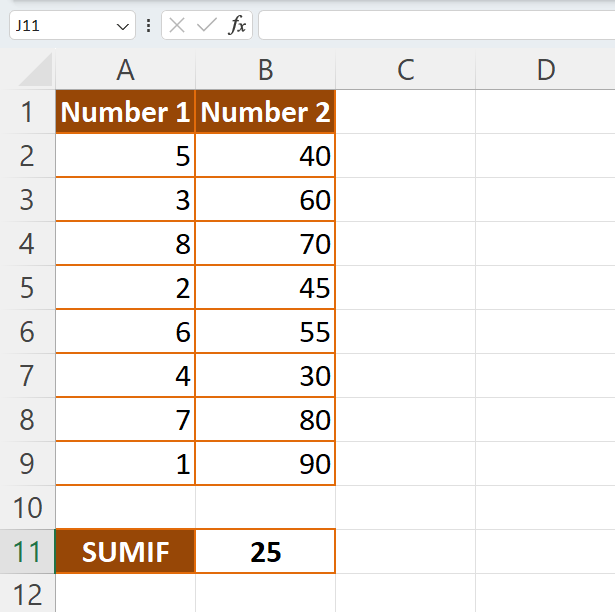
When it finds a match (in cells B2, B3, B5, B7, and B8), it considers the corresponding value from the "Number 1" column (A2 to A9).
The formula evaluates each cell in the "Number 2" column (B2 to B9) one by one.
It checks if the value in the "Number 2" column is greater than 50, as specified by the condition ">50."
It adds up all the values from the "Number 1" column that correspond to a "Number 2" value greater than 50.

In your provided data, there are five pairs with "Number 2" values greater than 50, and their corresponding "Number 1" values are 3, 8, 6, 7, and 1. When you add these "Number 1" values together, you get a total of 25.

So, the result of the formula "=SUMIF(B2:B9,">50",A2:A9)" is 25, which represents the sum of "Number 1" values for pairs where the corresponding"Number 2" is greater than 50.

This formula is a useful tool for performing conditional sums in Excel or similar spreadsheet software. It allows you to calculate the sum of values based on specific conditions, providing a way to analyze data and extract meaningful insights.