Understanding the RATE Function in Excel: A Guide to Calculating Interest Rates

The RATE function is another financial function in Excel that is used to calculate the interest rate per period of a loan or investment, given the total number of payment periods, the periodic payment, the present value, and the future value. It is the inverse of the PMT function, which calculates the periodic payment given the interest rate per period, the total number of payment periods, the present value, and the future value.The syntax of the RATE function is as follows:

Syntax

=RATE(nper, pmt, pv, [fv], [type], [guess])

Where:

nper: This is the total number of payment periods for the loan or investment.
pmt: This is the periodic payment made for the loan or investment.
pv: This is the present value of the loan or investment.
[fv] (optional):This is the future value of the loan or investment. If this parameter is not specified, then Excel assumes that the future value is zero.
[type] (optional):This parameter specifies when payments are due. If payments are due at the beginning of the period, then type should be set to 1. If payments are due at the end of the period, then type should be set to 0 or omitted.
guess (optional): This parameter is an estimate of the interest rate. If this parameter is not specified, then Excel assumes a default value of 0.1 (or 10%).

The RATE function returns the interest rate per period of the loan or investment as a decimal. This value can be multiplied by the number of periods per year to get the annual interest rate.

For example

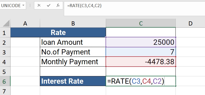
=RATE(C3,C4,C2)

The formula =RATE(C3,C4,C2) is an example of how to use the RATE function in Excel. Here is what each of the parameters represents:

C3 This is the total number of payment periods for the loan or investment. This value should be entered as a positive integer or reference to a cell containing a positive integer. For example, if the loan has a term of 7 years with monthly payments.
C4This is the periodic payment made for the loan or investment. This value should be entered as a negative number or a reference to a cell containing a negative number, since payments represent cash outflows. For example, if the monthly payment on a loan is $4478.38, you would enter -4478.38 or a reference to a cell containing -4478.38.
C2This is the present value of the loan or investment. This value should be entered as a positive number or reference to a cell containing a positive number. For example, if you are borrowing $25,000, you would enter 10000 or a reference to a cell containing 25000.