NPER Function in Excel: How to Calculate the Number of Payment Periods

The NPER function in Excel is a financial function that is used to calculate the number of payment periods required to pay off a loan or investment, based on a fixed interest rate, periodic payments, and a specified present value or future value. The syntax for the NPER function is:

Syntax

=NPER(rate, pmt, pv, [fv], [type])

Where:

rate: The interest rate per period of the loan or investment.
pmt: The periodic payment made for the loan or investment. This value should be entered as a negative number, since payments represent cash outflows.
pv: The present value of the loan or investment.
[fv] (optional): The future value of the loan or investment. If omitted, this argument is assumed to be 0.
[type] (optional): A value that specifies when payments are due. If omitted, this argument is assumed to be 0 (payments are due at the end of each period). Use 1 to indicate that payments are due at the beginning of each period.

The NPER function returns the number of payment periods required to pay off the loan or investment, based on the specified inputs. This value represents the total number of payments made over the entire term of the loan or investment.

Example

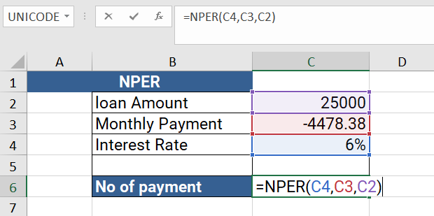
=NPER(C4,C3,C2)

The formula =NPER(C4,C3,C2) is an Excel formula that uses the NPER function to calculate the number of payment periods required to pay off a loan or investment, based on a fixed interest rate, periodic payments, and a specified present value.

Here's what each of the arguments in the formula represents:

C4: This is the interest rate per period of the loan or investment. It should be entered as a decimal, not a percentage. For example, if the annual interest rate is 6%, you would enter 0.06/12 if payments are made monthly.
C3: This is the periodic payment made for the loan or investment. It should be entered as a negative number, since payments represent cash outflows. For example, if the monthly payment is $4478.38, you would enter -4478.38.
C2:This is the present value of the loan or investment. It represents the initial amount borrowed or invested. For example, if you borrowed $25,000, you would enter 25000.

When you enter the formula into a cell in Excel, it will calculate the number of payment periods required to pay off the loan or investment, based on the specified inputs. The result will be displayed in the cell where the formula is entered.

It's important to note that the NPER function assumes that the interest rate, payment amount, and present value will remain constant over the entire payment period. If any of these values change, the actual number of payment periods required to pay off the loan or investment may be different from the result calculated by the NPER function.