Understanding the Index Function in Excel

The Index function in Excel is a powerful and versatile function used for retrieving data from a specific location within an array or range. It allows you to extract a value or an array of values based on specified row and column indices.

Syntax

=INDEX(array, row_num, [column_num])

"array" refers to the range of cells or an array from which you want to retrieve data.
"row_num" is the row number within the array that you want to reference.
"column_num" (optional) is the column number within the array that you want to reference. If omitted, the Index function will return the entire row specified by "row_num".

The Index function can be used in various scenarios, such as:

Single Cell Retrieval: If you specify both the row and column numbers, the function returns the value at the intersection of the specified row and column within the array.
Entire Row or Column Retrieval: If you omit the column number, the function returns the entire row specified by the row number as an array of values.
Multiple Cell Retrieval:By combining the Index function with other functions, such as the Match function, you can dynamically retrieve multiple cells from a range based on specific criteria or conditions.

The Index function is often used in combination with other functions like Match, If, or functions that perform calculations or conditional logic. It provides flexibility in extracting and manipulating data within Excel worksheets, making it a valuable tool for data analysis, reporting, and automation tasks.

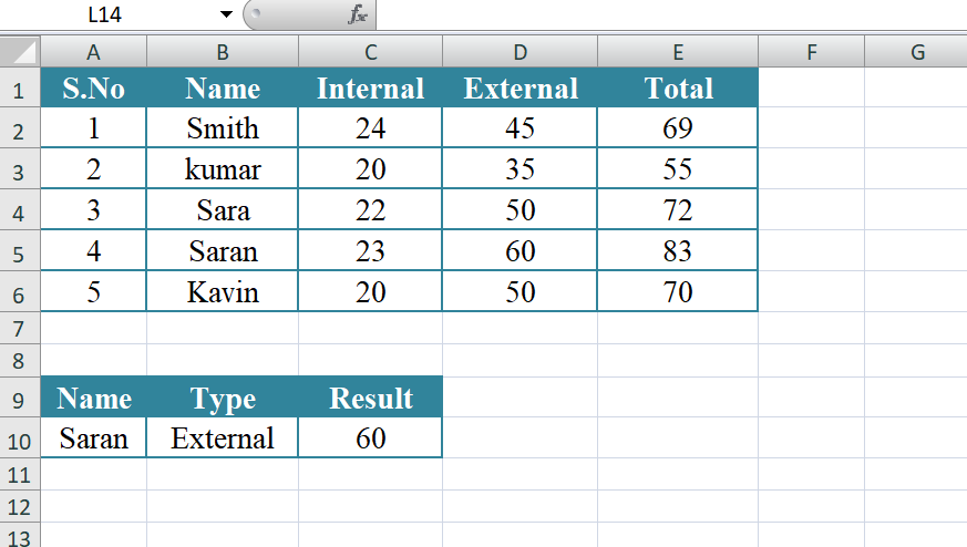
In the given example, we have a table that represents the scores of different individuals in three categories: Internal, External, and Total. The names of the individuals are listed in column A, and the scores are recorded in columns B, C, and D.

To retrieve a specific score from the table using the Index function, we can use the following formula:

=INDEX(C2:E7, MATCH(A10, B2:B7, 0), MATCH(B10, C1:E1, 0))

Let's break down the formula:

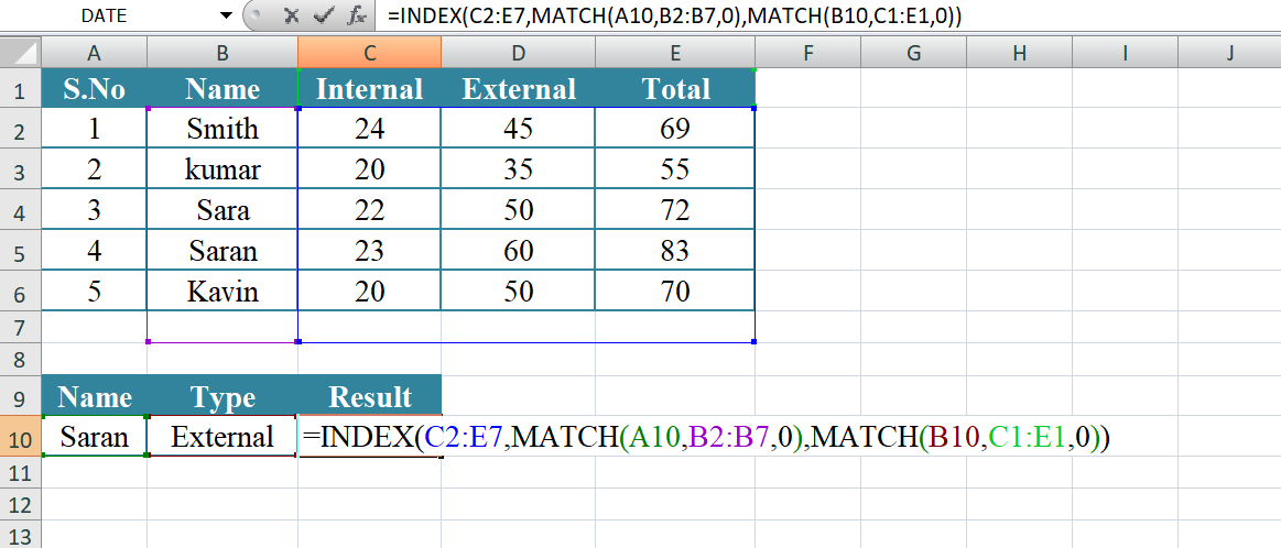
INDEX(C2:E7, ...) - This specifies the range or array from which we want to retrieve the data. In this case, we select the range C2:E7, which corresponds to the scores in the Internal, External, and Total columns.
MATCH(A10, B2:B7, 0) - This part of the formula finds the position of the value in cell A10 (which represents the name we want to match) within the range B2:B7 (the names column). The match type is set to 0, indicating an exact match.
MATCH(B10, C1:E1, 0) - This part determines the position of the value in cell B10 (which represents the category we want to match) within the range C1:E1 (the category headings). Again, the match type is set to 0 for an exact match.

By combining the Index function with two Match functions, we can dynamically retrieve the score from the table based on the specified name and category. The formula returns the corresponding score for the name and category combination.

For example, if we input "Sara" in cell A10 and "External" in cell B10, the formula will retrieve the score of 50, as it matches the name "Sara" in the names column and the category "External" in the category headings row.