Single Word Reverse Text Splitting in Excel
Single Word Reverse Text Splitting in Excel is a method of splitting a single word in Excel and reversing the order of its letters using formulas. This technique involves a combination of string manipulation formulas such as LEFT, RIGHT, MID, and LEN, along with the ampersand (&) operator to concatenate the results.
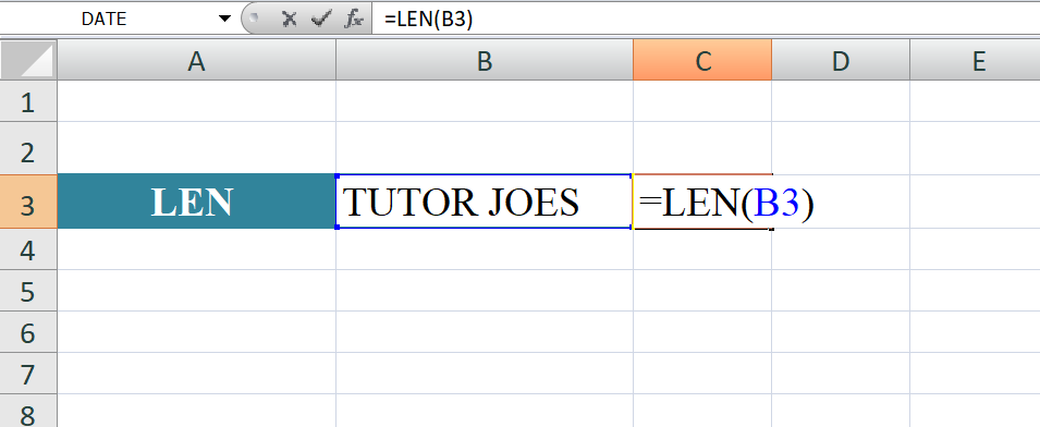
The LEN formula with the text "Tutor Joes", here it is:
Let's assume that cell A2 contains the text "Tutor Joes".
To calculate the length of the text in cell A2, you can use the formula:
SYNTAX
=LEN(A2)
In this case, the formula will return 10, as there are 10 characters in the phrase "Tutor Joes", including spaces.
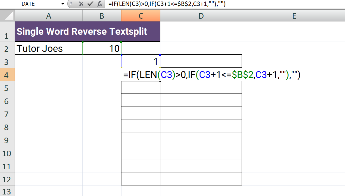
The formula you provided is an Excel formula that uses the IF function along with the LEN function to check if the length of the value in cell D3 is greater than 0. If it is, it then checks if the value in cell D3 plus 1 is less than or equal to the value in cell B2. If both conditions are true, it returns the value in cell D3 plus 1. Otherwise, it returns an empty string ("").
SYNTAX
=IF(LEN(D3)>0, IF(D3+1<=$B$2, D3+1, ""), "")
Here are the steps to perform Single Word Reverse Text Splitting in Excel:
- Select a cell where you want to display the reversed word.
- Enter the word you want to reverse in another cell (e.g., cell A1).
- Determine the length of the word using the LEN function, which returns the number of characters in a text string. For example, you can use the formula =LEN(A1) to determine the length of the word in cell A1.
- Use the RIGHT function to extract the rightmost character of the word, starting from the last character, and concatenate it with the other characters. For example, you can use the formula =RIGHT(A1,1) & "" to extract the last character of the word in cell A1 and concatenate it with an empty string (""), which forces Excel to treat the result as text.
- Repeat step 4 for the remaining characters in the word, using the MID function to extract the middle characters, and the LEFT function to extract the first character. For example, you can use the formula =MID(A1,LEN(A1)-1,1) & "" to extract the second-to-last character of the word, and the formula =LEFT(A1,1) & "" to extract the first character of the word.
- Concatenate the results of the previous steps using the ampersand (&) operator to form the reversed word. For example, you can use the formula =RIGHT(A1,1) & "" & MID(A1,LEN(A1)-1,1) & "" & LEFT(A1,1) & "" to reverse the word in cell A1.
For example
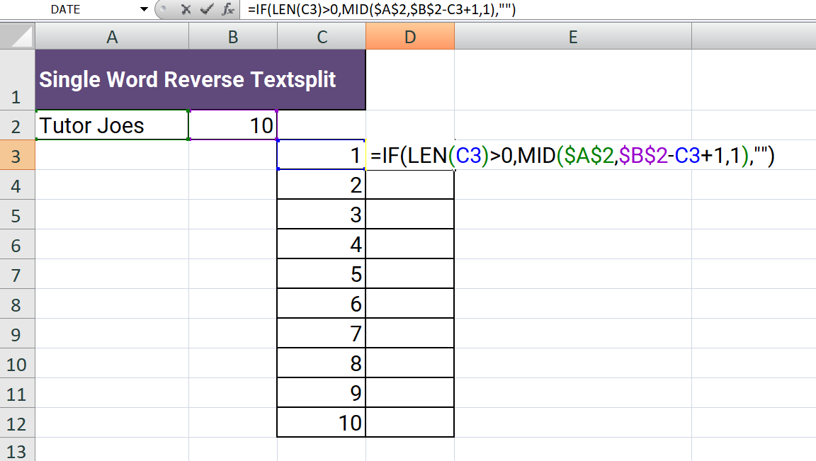
=IF(LEN(C3)>0,MID($A$2,$B$2-C3+1,1),"")
The formula=IF(LEN(C3)>0,MID($A$2,$B$2-C3+1,1),"") can be used to extract a single character from a text string based on a specific position or index. In the context of the "Tutor Joes" example, this formula can be used to extract the first letter of each name in the list, starting with the last letter and moving leftward.
the different parts of the formula as it applies to the "Tutor Joes" example:
- IF: This is an Excel logical function that evaluates a condition and returns one value if the condition is true and another value if it is false.
- LEN: This is an Excel function that returns the length of a text string.
- C3: This is the cell reference that contains the index or position of the character to extract from the text string.
- MID: This is an Excel function that returns a specified number of characters from a text string, starting at a specified position.
- $A$2: This is the cell reference that contains the text string to extract a character from.
- $B$2: This is the cell reference that contains the position of the last character in the text string.
- 1: This specifies the number of characters to extract from the text string, which in this case is just one.
- "": This is the value to return if the condition in the IF statement is false, which in this case is an empty string.
In the "Tutor Joes" example, cell A1 contains the name "Tutor Joes", while cell B1 contains the length of the name (10). The formula =IF(LEN(C3)>0,MID($A$2,$B$2-C3+1,1),"")is entered into cell E1, with cell C3 containing the formula "=ROW()-1". The formula in cell C3 returns a sequence of numbers from 0 to 9, which are used as indices to extract the individual characters of the name from right to left.
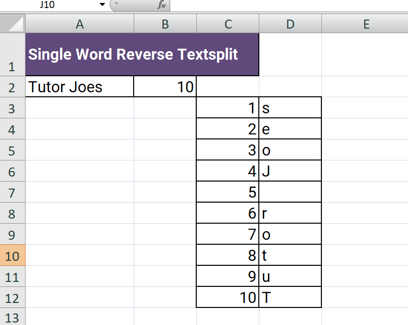
Output
Learn All in Tamil © Designed & Developed By Tutor Joes | Privacy Policy | Terms & Conditions